Quickstart

This notebook is intended to quickly demonstrate some use cases for rousepull. The structure is as follows:

• set up some dummy data; in a real application this would of course be replaced by real data

• run inference to get a qualitative force profile

• calibrate the inference to get quantitative results

• apply the dragging models used in the original paper

import numpy as np
from matplotlib import pyplot as plt

import rousepull

np.random.seed(18673550)

Generate dummy data

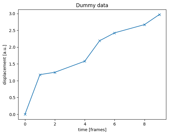
t = np.arange(10)           # equally spaced frame numbers
t = np.delete(t, [3, 7])    # remove some frames for illustration
                            # Note: the data (`x` below) should not contain np.nan;
                            # just remove the corresponding entry instead

x = np.sqrt(t)                         # for constant force we expect x ~ √t
x += 0.2*np.random.normal(size=len(x)) # add some noise
x -= x[0]                              # for visualization it is nice to have x[0] = 0
                                       # (this is not required for the inference)

# Plot
plt.plot(t, x, marker='x')
plt.xlabel('time [frames]')
plt.ylabel('displacement [a.u.]')
plt.title('Dummy data')
plt.show()

Run inference

inf = rousepull.ForceInference(t, x) # set up inference object
inf.populate()                       # run the inference
                                     # the inferred force profile is now stored in inf.fpoly

# Plot
plt.plot(t, x, marker='x', label='x(t)')              # plot input trajectory
fplot = inf.fpoly[list(range(len(inf.fpoly))) + [-1]] # duplicate last element for plotting
plt.step(inf.tf, fplot, where='post', label='f(t)')   # plot inferred force profile

plt.legend()
plt.xlabel('time [frames]')
plt.ylabel('displacement [a.u.] // force [a.u.]')
plt.title('Dummy data with inference')
plt.show()

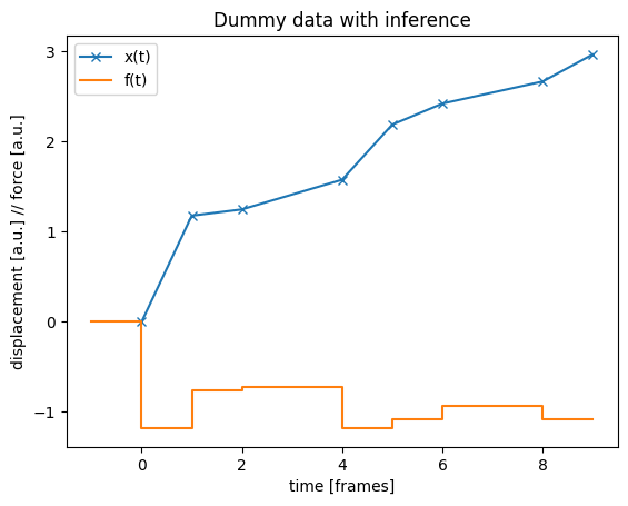
Notes:

• the inferred force is negative, since this is the restoring force exerted by the polymer on the locus.

• the plot shows how the inference works with the discretization inherent to the data: the force is assumed to be constant between measurements, and identically equal to zero before the first one.

• overall, the inference shows a constant force of about -1, consistent with how the dummy data were generated (x = √t + noise).

Calibration

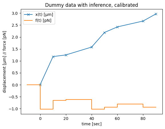
To make the force inference quantitative, we need to calibrate the conversion factor between time and length scales (note that above we wrote x(t) = √t, which of course does not make sense in physical units). To that end, we use the MSD prefactor from the force free situation.

In the absence of pulling force, the locus under consideration should undergo Rouse diffusion, i.e. exhibit an MSD ⟨x²(t)⟩ = Γ√t. We can use this prefactor Γ to calibrate the inference; it is simply passed as parameter to the constructor.

For this example, let’s assume that the lag time between successive frames is 10s, and the locus moves with Γ = 0.003 μm²/√s in the absence of force, while the measured displacement x(t) is in μm already. The inference then gives the force profile in pN:

dt = 10       # sec / frame
Gamma = 0.003 # μm² / √s

inf = rousepull.ForceInference(t*dt,        # time is now in seconds
                               x,           # μm
                               Gamma=Gamma, # μm² / √s
                              )
inf.populate()

# Plot
plt.plot(inf.t, inf.x, marker='x', label='x(t) [μm]')
fplot = inf.fpoly[list(range(len(inf.fpoly))) + [-1]]
plt.step(inf.tf, fplot, where='post', label='f(t) [pN]')

plt.legend()
plt.xlabel('time [sec]')
plt.ylabel('displacement [μm] // force [pN]')
plt.title('Dummy data with inference, calibrated')
plt.show()

Dragging surrounding material

In the original publication we inserted additional hindrance to the locus motion due to dragging surrounding material. This can work in a few different ways, for this example let us assume that some of the chromatin the locus moves through sticks to it. This generates an additional force component, that can be calculated using the computeFdrag() function.

# using the inference object inf from previous example
inf.computeFdrag(density=0.2*np.ones(len(inf.t)), # attachment parameter; can be different along the
                                                  # trajectory, e.g. proportional to observed DNA density
                 mode=0,                          # which dragging model to use; see docstring
                )

# Plotting
plt.plot(inf.t, inf.x, marker='x', label='x(t) [μm]')
fplot = inf.fpoly[list(range(len(inf.fpoly))) + [-1]]
plt.step(inf.tf, fplot, where='post', label='polymer force [pN]')
fplot = inf.fdrag[list(range(len(inf.fdrag))) + [-1]]
plt.step(inf.tf, fplot, where='post', label='dragging force [pN]')
fplot = inf.fpoly + inf.fdrag
fplot = fplot[list(range(len(fplot))) + [-1]]
plt.step(inf.tf, fplot, where='post', label='total force [pN]')

plt.legend()
plt.xlabel('time [sec]')
plt.ylabel('displacement [μm] // force [pN]')
plt.title('Dummy data with inference + dragging, calibrated')
plt.show()

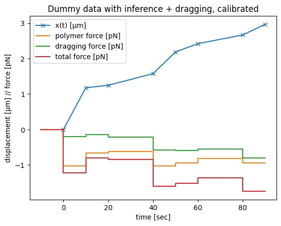
To interpret this plot, remember that we observe the blue trajectory and then ask what force would be necessary to move the locus as observed. Since we work in the overdamped limit, the total force pulling the locus forward has to exactly compensate the different restoring components. These restoring forces can be due to

• viscous friction, i.e. proportional to locus velocity (not shown, since we usually find this component to be negligible)

• the polymer pulling the locus back (orange)

• surrounding chromatin sticking to the locus as it moves (green)

So if there is sticky chromatin, the total force needed (red) to move the locus as observed (blue) is larger than without this additional hindrance (orange).